一个图模型包含 N N N x ‾ = ( x 1 , … , x N ) \underline{x}=(x_1,\dots,x_N) x = ( x 1 , … , x N ) X \mathcal{X} X
给定一些条件,求另一些变量的边缘分布;
一些后验估计相关
但是我们不会去直接计算联合分布 p ( x ‾ ) p(\underline{x}) p ( x ) ∣ X ∣ N |\mathcal{X}|^N ∣ X ∣ N
Example 1: Ising chain
Ferromagnetic Ising model has σ ‾ = ( σ 1 , … , σ N ) , σ i ∈ { 1 , − 1 } \underline{\sigma}=(\sigma_1,\dots, \sigma_N), \sigma_i\in\{1,-1\} σ = ( σ 1 , … , σ N ) , σ i ∈ { 1 , − 1 }
μ β ( σ ‾ ) = 1 Z exp ( β ∑ i = 1 N − 1 σ i σ i + 1 + β B ∑ i = 1 N σ i ) \mu_\beta(\underline{\sigma}) = \frac{1}{Z} \exp\left(\beta \sum_{i=1}^{N-1} \sigma_i \sigma_{i+1}+\beta B\sum_{i=1}^N\sigma_i\right)
μ β ( σ ) = Z 1 exp ( β i = 1 ∑ N − 1 σ i σ i + 1 + βB i = 1 ∑ N σ i )
where Z Z Z
我们计算 σ j \sigma_j σ j ∝ \propto ∝
μ ( σ j ) ∝ ∑ σ 1 , … , σ j − 1 , σ j + 1 , … , σ N exp ( β ∑ i = 1 N − 1 σ i σ i + 1 + β B ∑ i = 1 N σ i ) = ∑ σ 1 , … , σ j − 1 , σ j + 1 , … , σ N exp ( β ∑ i = 1 j − 1 σ i σ i + 1 + β B ∑ i = 1 j − 1 σ i ) exp ( β ∑ i = j N − 1 σ i σ i + 1 + β B ∑ i = j + 1 N σ i ) exp ( β B σ j ) \mu(\sigma_j)\propto\sum_{\sigma_1,\dots,\sigma_{j-1},\sigma_{j+1},\dots,\sigma_{N}}\exp\left(\beta \sum_{i=1}^{N-1} \sigma_i \sigma_{i+1}+\beta B\sum_{i=1}^N\sigma_i\right)
\\=\sum_{\sigma_1,\dots,\sigma_{j-1},\sigma_{j+1},\dots,\sigma_{N}}\exp\left(\beta \sum_{i=1}^{j-1} \sigma_i \sigma_{i+1}+\beta B\sum_{i=1}^{j-1}\sigma_i\right)\exp\left(\beta\sum_{i=j}^{N-1} \sigma_i \sigma_{i+1}+\beta B\sum_{i=j+1}^{N}\sigma_i\right)\exp\left(\beta B\sigma_{j}\right) μ ( σ j ) ∝ σ 1 , … , σ j − 1 , σ j + 1 , … , σ N ∑ exp ( β i = 1 ∑ N − 1 σ i σ i + 1 + βB i = 1 ∑ N σ i ) = σ 1 , … , σ j − 1 , σ j + 1 , … , σ N ∑ exp ( β i = 1 ∑ j − 1 σ i σ i + 1 + βB i = 1 ∑ j − 1 σ i ) exp ( β i = j ∑ N − 1 σ i σ i + 1 + βB i = j + 1 ∑ N σ i ) exp ( βB σ j )
分配拆开即可,是两个和的乘积. 定义 "message":
$$\begin{aligned}
\widehat\nu_{\to j}(\sigma_j) &= \frac{1}{Z_{\to j}} \sum_{\sigma_1\dots\sigma_{j-1}}
\exp\left\{\beta \sum_{i=1}^{j-1}\sigma_i\sigma_{i+1} + \beta B \sum_{i=1}^{j-1}\sigma_i\right\}, \\[4pt]
\widehat\nu_{j\leftarrow}(\sigma_j) &= \frac{1}{Z_{j\leftarrow}} \sum_{\sigma_{j+1}\dots\sigma_N}
\exp\left\{\beta \sum_{i=j}^{N-1}\sigma_i\sigma_{i+1} + \beta B \sum_{i=j+1}^{N}\sigma_i\right\}.
\end{aligned}$$
$$\mu(\sigma_j) \;\cong\; \widehat\nu_{\to j}(\sigma_j)\,
e^{\beta B\sigma_j}\, \widehat\nu_{j\leftarrow}(\sigma_j) .$$
This decomposition is interesting because the various messages can be computed iteratively.
而这两个部分都是 local 信息,左边的求和和右边无关. 例如 ν ^ → 1 ( σ 1 ) \hat{\nu}_{\to1}(\sigma_1) ν ^ → 1 ( σ 1 ) ν ^ ← n ( σ n ) \hat{\nu}_{\leftarrow n}(\sigma_n) ν ^ ← n ( σ n )
ν ^ → i ( σ i ) ∝ ∑ σ i − 1 ν ^ → ( i − 1 ) ( σ i − 1 ) exp ( β σ i − 1 σ i + β B σ i − 1 ) \hat{\nu}_{\to i}(\sigma_i)
\propto \sum_{\sigma_{i-1}} \hat{\nu}_{\to(i-1)}(\sigma_{i-1})
\exp\!\left( \beta \, \sigma_{i-1}\sigma_i +\beta B \sigma_{i-1}\right) ν ^ → i ( σ i ) ∝ σ i − 1 ∑ ν ^ → ( i − 1 ) ( σ i − 1 ) exp ( β σ i − 1 σ i + βB σ i − 1 )
ν ^ ← i ( σ i ) ∝ ∑ σ i + 1 ν ^ ← ( i + 1 ) ( σ i + 1 ) exp ( β σ i σ i + 1 + β B σ i + 1 ) \hat{\nu}_{\leftarrow i}(\sigma_i)
\propto \sum_{\sigma_{i+1}} \hat{\nu}_{\leftarrow(i+1)}(\sigma_{i+1})
\exp\!\left( \beta \, \sigma_{i}\sigma_{i+1} +\beta B \sigma_{i+1}\right) ν ^ ← i ( σ i ) ∝ σ i + 1 ∑ ν ^ ← ( i + 1 ) ( σ i + 1 ) exp ( β σ i σ i + 1 + βB σ i + 1 )
Example 2. a tree-parity-check code
We start from a concrete example.
$$x_0 \oplus x_1 \oplus x_2 = \mathsf{0},$$
$$x_0 \oplus x_3 \oplus x_4 = \mathsf{0},$$
$$x_0 \oplus x_5 \oplus x_6 = \mathsf{0}.$$
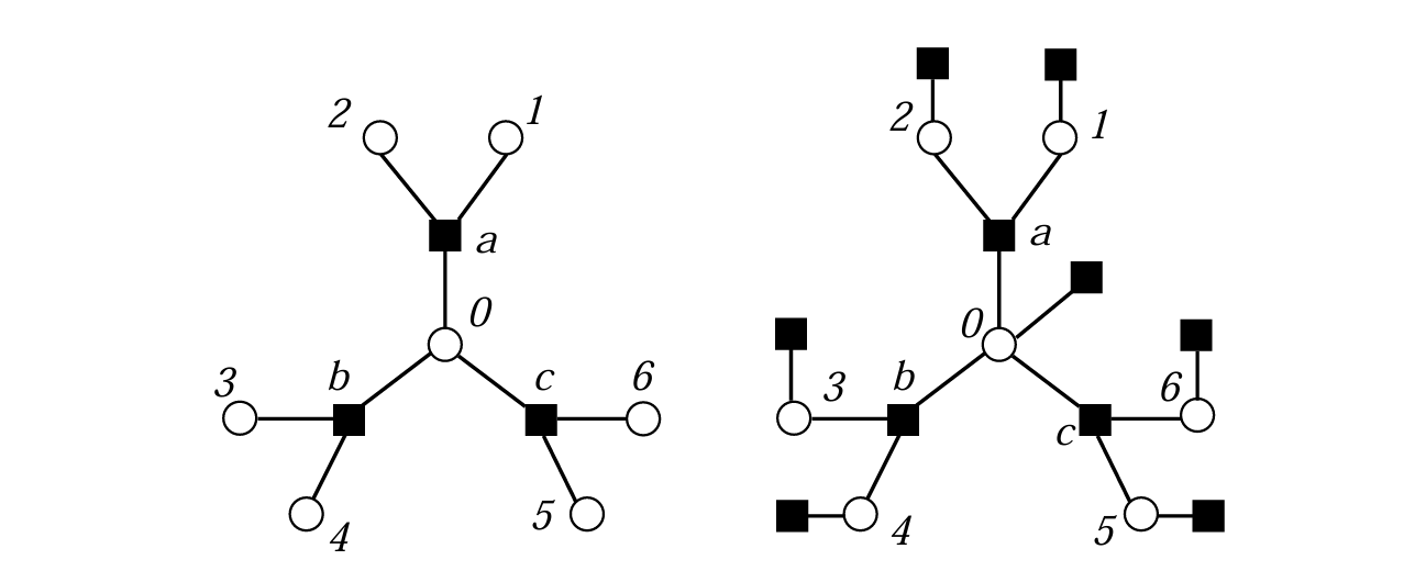
Fig. 14.2 — Left: a simple parity check code with 7 variables and 3 checks. Right: the factor graph corresponding to the problem of finding the sent codeword, given a received message.
左图是这个方程组的 factor graph.
已知纠错矩阵,将一个 x x x p p p p p p y y y y y y Q ( i ∣ i ) = 1 − p , Q ( i ∣ j ) = p , ∀ i ≠ j Q(i|i)=1-p,Q(i|j)=p,\forall\;i\neq j Q ( i ∣ i ) = 1 − p , Q ( i ∣ j ) = p , ∀ i = j
$$\mu_y(\underline{x}) \;\cong\;
\mathbb{I}(x_0\oplus x_1\oplus x_2 = \mathsf{0})\,
\mathbb{I}(x_0\oplus x_3\oplus x_4 = \mathsf{0})\,
\mathbb{I}(x_0\oplus x_5\oplus x_6 = \mathsf{0})
\prod_{i=0}^{6} Q(y_i \mid x_i) ,$$
我们可以逐 bit 分析,需要在给定 y y y x i x_i x i y = ( 1000010 ) y=(1000010) y = ( 1000010 )
μ ( x 1 ) ∝ ∑ x 0 x 2 , … , x 6 I ( x 0 ⊕ x 1 ⊕ x 2 = 0 ) I ( x 0 ⊕ x 3 ⊕ x 4 = 0 ) I ( x 0 ⊕ x 5 ⊕ x 6 = 0 ) ∏ i = 0 6 Q ( y i ∣ x i ) = ∑ x 0 , x 2 I ( x 0 ⊕ x 1 ⊕ x 2 = 0 ) Q ( y 0 ∣ x 0 ) Q ( y 2 ∣ x 2 ) × ∑ x 3 , x 4 I ( x 0 ⊕ x 3 ⊕ x 4 = 0 ) Q ( y 3 ∣ x 3 ) Q ( y 4 ∣ x 4 ) × ∑ x 5 , x 6 I ( x 0 ⊕ x 5 ⊕ x 6 = 0 ) Q ( y 5 ∣ x 5 ) Q ( y 6 ∣ x 6 ) × Q ( y 1 ∣ x 1 ) = Q ( y 1 ∣ x 1 ) ∑ x 0 , x 2 I ( x 0 ⊕ x 1 ⊕ x 2 = 0 ) Q ( y 0 ∣ x 0 ) Q ( y 2 ∣ x 2 ) ν ^ b → 0 ( x 0 ) ν ^ c → 0 ( x 0 ) \mu(x_1)\propto\sum_{x_0x_2,\dots,x_6}
\mathbb{I}(x_{0} \oplus x_{1} \oplus x_{2} = 0)\,
\mathbb{I}(x_{0} \oplus x_{3} \oplus x_{4} = 0)\,
\mathbb{I}(x_{0} \oplus x_{5} \oplus x_{6} = 0)\,
\prod_{i=0}^{6} Q(y_i | x_i) \,\\
=\sum_{x_0,x_2}\mathbb{I}(x_{0} \oplus x_{1} \oplus x_{2} = 0)Q(y_0|x_0)Q(y_2|x_2)\\\times
\sum_{x_3,x_4}\mathbb{I}(x_{0} \oplus x_{3} \oplus x_{4} = 0)Q(y_3|x_3)Q(y_4|x_4)\\\times
\sum_{x_5,x_6}\mathbb{I}(x_{0} \oplus x_{5} \oplus x_{6} = 0)Q(y_5|x_5)Q(y_6|x_6)\\\times
Q(y_1 | x_1) \, \\
= Q(y_1|x_1) \sum_{x_0,x_2}\mathbb{I}(x_{0} \oplus x_{1} \oplus x_{2} = 0)Q(y_0|x_0)Q(y_2|x_2)\hat{\nu}_{b\to0}(x_0)\hat{\nu}_{c\to0}(x_0)
μ ( x 1 ) ∝ x 0 x 2 , … , x 6 ∑ I ( x 0 ⊕ x 1 ⊕ x 2 = 0 ) I ( x 0 ⊕ x 3 ⊕ x 4 = 0 ) I ( x 0 ⊕ x 5 ⊕ x 6 = 0 ) i = 0 ∏ 6 Q ( y i ∣ x i ) = x 0 , x 2 ∑ I ( x 0 ⊕ x 1 ⊕ x 2 = 0 ) Q ( y 0 ∣ x 0 ) Q ( y 2 ∣ x 2 ) × x 3 , x 4 ∑ I ( x 0 ⊕ x 3 ⊕ x 4 = 0 ) Q ( y 3 ∣ x 3 ) Q ( y 4 ∣ x 4 ) × x 5 , x 6 ∑ I ( x 0 ⊕ x 5 ⊕ x 6 = 0 ) Q ( y 5 ∣ x 5 ) Q ( y 6 ∣ x 6 ) × Q ( y 1 ∣ x 1 ) = Q ( y 1 ∣ x 1 ) x 0 , x 2 ∑ I ( x 0 ⊕ x 1 ⊕ x 2 = 0 ) Q ( y 0 ∣ x 0 ) Q ( y 2 ∣ x 2 ) ν ^ b → 0 ( x 0 ) ν ^ c → 0 ( x 0 )
μ ( x 0 ) ∝ ∑ x 1 , … , x 6 I ( x 0 ⊕ x 1 ⊕ x 2 = 0 ) I ( x 0 ⊕ x 3 ⊕ x 4 = 0 ) I ( x 0 ⊕ x 5 ⊕ x 6 = 0 ) ∏ i = 0 6 Q ( y i ∣ x i ) = ∑ x 1 , x 2 I ( x 0 ⊕ x 1 ⊕ x 2 = 0 ) Q ( y 1 ∣ x 1 ) Q ( y 2 ∣ x 2 ) × ∑ x 3 , x 4 I ( x 0 ⊕ x 3 ⊕ x 4 = 0 ) Q ( y 3 ∣ x 3 ) Q ( y 4 ∣ x 4 ) × ∑ x 5 , x 6 I ( x 0 ⊕ x 5 ⊕ x 6 = 0 ) Q ( y 5 ∣ x 5 ) Q ( y 6 ∣ x 6 ) × Q ( y 0 ∣ x 0 ) \mu(x_0)\propto\sum_{x_1,\dots,x_6}
\mathbb{I}(x_{0} \oplus x_{1} \oplus x_{2} = 0)\,
\mathbb{I}(x_{0} \oplus x_{3} \oplus x_{4} = 0)\,
\mathbb{I}(x_{0} \oplus x_{5} \oplus x_{6} = 0)\,
\prod_{i=0}^{6} Q(y_i | x_i) \, \\
=\sum_{x_1,x_2}\mathbb{I}(x_{0} \oplus x_{1} \oplus x_{2} = 0)Q(y_1|x_1)Q(y_2|x_2)\\\times
\sum_{x_3,x_4}\mathbb{I}(x_{0} \oplus x_{3} \oplus x_{4} = 0)Q(y_3|x_3)Q(y_4|x_4)\\\times
\sum_{x_5,x_6}\mathbb{I}(x_{0} \oplus x_{5} \oplus x_{6} = 0)Q(y_5|x_5)Q(y_6|x_6)\\\times
Q(y_0 | x_0) \,
μ ( x 0 ) ∝ x 1 , … , x 6 ∑ I ( x 0 ⊕ x 1 ⊕ x 2 = 0 ) I ( x 0 ⊕ x 3 ⊕ x 4 = 0 ) I ( x 0 ⊕ x 5 ⊕ x 6 = 0 ) i = 0 ∏ 6 Q ( y i ∣ x i ) = x 1 , x 2 ∑ I ( x 0 ⊕ x 1 ⊕ x 2 = 0 ) Q ( y 1 ∣ x 1 ) Q ( y 2 ∣ x 2 ) × x 3 , x 4 ∑ I ( x 0 ⊕ x 3 ⊕ x 4 = 0 ) Q ( y 3 ∣ x 3 ) Q ( y 4 ∣ x 4 ) × x 5 , x 6 ∑ I ( x 0 ⊕ x 5 ⊕ x 6 = 0 ) Q ( y 5 ∣ x 5 ) Q ( y 6 ∣ x 6 ) × Q ( y 0 ∣ x 0 )
乘积的第一项,就是指 x 0 x_0 x 0 { 0 , a , 1 , 2 } \{0,a,1,2\} { 0 , a , 1 , 2 } ν ^ a → 0 ( x 0 ) ∝ ∑ x 1 , x 2 I ( x 0 ⊕ x 1 ⊕ x 2 = 0 ) Q ( y 1 ∣ x 1 ) Q ( y 2 ∣ x 2 ) \hat{\nu}_{a\to0}(x_0)\propto\sum_{x_1,x_2}\mathbb{I}(x_{0} \oplus x_{1} \oplus x_{2} = 0)Q(y_1|x_1)Q(y_2|x_2) ν ^ a → 0 ( x 0 ) ∝ ∑ x 1 , x 2 I ( x 0 ⊕ x 1 ⊕ x 2 = 0 ) Q ( y 1 ∣ x 1 ) Q ( y 2 ∣ x 2 )
μ ( x 1 ) ∝ Q ( y 1 ∣ x 1 ) ν ^ a → 1 ( x 1 ) \mu(x_1)\propto Q(y_1|x_1)\hat{\nu}_{a\to1}(x_1)
μ ( x 1 ) ∝ Q ( y 1 ∣ x 1 ) ν ^ a → 1 ( x 1 )
μ ( x 0 ) ∝ Q ( y 0 ∣ x 0 ) ν ^ a → 0 ( x 0 ) ν ^ b → 0 ( x 0 ) ν ^ c → 0 ( x 0 ) \mu(x_0)\propto Q(y_0|x_0)\hat{\nu}_{a\to0}(x_0)\hat{\nu}_{b\to0}(x_0)\hat{\nu}_{c\to0}(x_0)
μ ( x 0 ) ∝ Q ( y 0 ∣ x 0 ) ν ^ a → 0 ( x 0 ) ν ^ b → 0 ( x 0 ) ν ^ c → 0 ( x 0 )
Belief Propagation on Trees
In this section,
μ ( x ‾ ) = 1 Z ψ a ( x ‾ ∂ a ) \mu(\underline{x})=\frac{1}{Z}\psi_a(\underline{x}_{\partial a}) μ ( x ) = Z 1 ψ a ( x ∂ a )
where ψ a \psi_a ψ a { x i : i ∈ ∂ a } \{x_i:i\in\partial a\} { x i : i ∈ ∂ a } a a a ∂ i \partial i ∂ i When the factor graph has no loop the following are among the basic problems
that can be solved efficiently with a message-passing procedure:
Compute the marginal distributions of one variable, $\mu(x_i)$, or the joint
distribution of a small number of variables.
Sample from $\mu(\underline{x})$, i.e. draw independent random configurations
$\underline{x}$ with distribution $\mu(\underline{x})$.
Compute the partition function $Z$, or equivalently, in statistical physics
language, the free-entropy $\log Z$.
We have BP rules:
ν j → a ( x j ) ≅ ∏ b ∈ ∂ j ∖ a ν ^ b → j ( x j ) ν ^ a → j ( x j ) ≅ ∑ x ‾ ∂ a ∖ j ψ a ( x ‾ ∂ a ) ∏ k ∈ ∂ a ∖ j ν k → a ( x k ) . \nu_{j \to a}(x_j) \;\cong\; \prod_{b \in \partial j \setminus a}
\hat{\nu}_{b \to j}(x_j)\\
\hat{\nu}_{a \to j}(x_j) \;\cong\;
\sum_{\underline{x}_{\partial a \setminus j}}
\psi_a(\underline{x}_{\partial a}) \prod_{k \in \partial a \setminus j}
\nu_{k \to a}(x_k). ν j → a ( x j ) ≅ b ∈ ∂ j ∖ a ∏ ν ^ b → j ( x j ) ν ^ a → j ( x j ) ≅ x ∂ a ∖ j ∑ ψ a ( x ∂ a ) k ∈ ∂ a ∖ j ∏ ν k → a ( x k ) .
Simple computation is able to show that the example of parity check code is consistent with the equations above.
If j j j 1 1 1 a a a ν j → a ( x j ) ∝ 1 \nu_{j \to a}(x_j)\propto1 ν j → a ( x j ) ∝ 1
Let us verify ν ^ a → 0 ( x 0 ) ∝ ∑ x 1 , x 2 I ( x 0 ⊕ x 1 ⊕ x 2 = 0 ) Q ( y 1 ∣ x 1 ) Q ( y 2 ∣ x 2 ) \hat{\nu}_{a\to0}(x_0)\propto\sum_{x_1,x_2}\mathbb{I}(x_{0} \oplus x_{1} \oplus x_{2} = 0)Q(y_1|x_1)Q(y_2|x_2) ν ^ a → 0 ( x 0 ) ∝ ∑ x 1 , x 2 I ( x 0 ⊕ x 1 ⊕ x 2 = 0 ) Q ( y 1 ∣ x 1 ) Q ( y 2 ∣ x 2 )
LHS = ∑ x 1 , x 2 I ( x 0 ⊕ x 1 ⊕ x 2 = 0 ) Q ( y 1 ∣ x 1 ) Q ( y 2 ∣ x 2 ) ∏ k = 1 , 2 ν k → a ( x k ) \text{LHS}=\sum_{x_1,x_2}\mathbb{I}(x_{0} \oplus x_{1} \oplus x_{2} = 0)Q(y_1|x_1)Q(y_2|x_2)\prod_{k=1,2}\nu_{k\to a}(x_k) LHS = ∑ x 1 , x 2 I ( x 0 ⊕ x 1 ⊕ x 2 = 0 ) Q ( y 1 ∣ x 1 ) Q ( y 2 ∣ x 2 ) ∏ k = 1 , 2 ν k → a ( x k )
A graph:
and a clarifying lecnote :
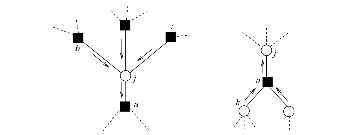
Fig. 14.3 — Left: portion of the factor graph involved in the computation of $\nu^{(t+1)}_{j\to a}(x_j)$; this message is a function of the incoming messages $\widehat\nu^{(t)}_{b\to j}(x_j)$, with $b \ne a$. Right: portion involved in the computation of $\widehat\nu^{(t)}_{a\to j}(x_j)$; a function of the incoming messages $\nu^{(t)}_{k\to a}(x_k)$, with $k \ne j$.
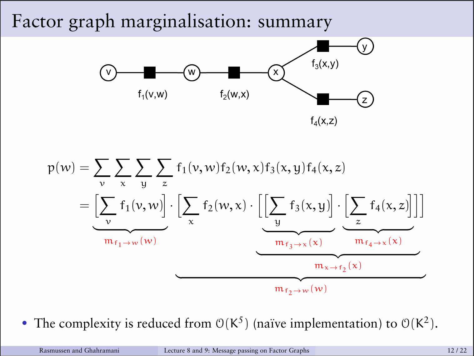
Factor graph marginalisation, worked through on one example — the braces tie each bracketed sum to the message it defines. Complexity drops from $\mathcal{O}(K^5)$ to $\mathcal{O}(K^2)$. (Rasmussen and Ghahramani, Message passing on Factor Graphs .)
实际上,以上的 BP 应该按照迭代的方式理解.
$$\nu^{(t+1)}_{j\to a}(x_j) \cong \prod_{b\in\partial j\setminus a}
\widehat\nu^{(t)}_{b\to j}(x_j), \tag{14.14}$$
$$\widehat\nu^{(t)}_{a\to j}(x_j) \cong \sum_{\underline{x}_{\partial a\setminus j}}
\psi_a(\underline{x}_{\partial a}) \prod_{k\in\partial a\setminus j} \nu^{(t)}_{k\to a}(x_k) . \tag{14.15}$$
这个有点像 Bellmann-ford, 明明我们要对整体进行分析(比如计算边缘分布)但是我们可以对局部(也就是每一条边)进行迭代得到结果.
We have converging theorem:
Theorem 14.1 — BP is exact on trees
Consider a tree-graphical model with diameter $t_*$ (which means that $t_*$ is
the maximum distance between any two variable nodes). Then
Irrespective of the initial condition, the BP update (14.14), (14.15) converges
after at most $t_*$ iterations. In other words, for any edge $(ia)$, and any
$t > t_*$,
$$\nu^{(t)}_{i\to a} = \nu^{*}_{i\to a}, \qquad
\widehat\nu^{(t)}_{a\to i} = \widehat\nu^{*}_{a\to i}.$$
The fixed point messages provide the exact marginals: for any variable node $i$,
and any $t > t_*$, $\nu^{(t)}_i(x_i) = \mu(x_i)$.
Correlations and Energy
现在我们更进一步,想要计算某两个变量的联合边缘分布 μ i j ( x i , x j ) \mu_{ij}(x_i,x_j) μ ij ( x i , x j ) μ ( x i ) \mu(x_i) μ ( x i ) P x ‾ ∼ μ ( x ‾ j = x j ∣ x ‾ i = x i ) \mathbb{P}_{\underline{x}\sim\mu}(\underline{x}_j=x_j|\underline{x}_i=x_i) P x ∼ μ ( x j = x j ∣ x i = x i ) x ‾ \underline{x} x
μ ( x ‾ ∣ x i = b ) ∝ ∏ a = 1 M ψ ( x ‾ ∂ a ) I ( x i = b ) . \mu(\underline{x}|x_i=b)\propto\prod_{a=1}^M\psi(\underline{x}_{\partial a})\mathbb{I}(x_i=b).
μ ( x ∣ x i = b ) ∝ a = 1 ∏ M ψ ( x ∂ a ) I ( x i = b ) .
其实相当于加一条约束 x i = b x_i=b x i = b i i i
记 F R F_R F R V R = ∂ F R V_R=\partial F_R V R = ∂ F R F R F_R F R R R R x ‾ R \underline{x}_R x R R R R R R R
根据 message 的物理意义,可以计算 x ‾ R \underline{x}_R x R ϕ a ( a ∈ F R ) \phi_a(a\in F_R) ϕ a ( a ∈ F R )
μ ( x ‾ R ) ∝ ∏ a ∈ F R ψ a ( x ‾ ∂ a ) ∏ a ∈ ∂ R ν ^ a → i ( a ) ( x i ( a ) ) \mu(\underline{x}_R)\propto\prod_{a\in F_R}\psi_a(\underline{x}_{\partial a})\prod_{a\in\partial R}\hat{\nu}_{a\to i(a)}(x_{i(a)})
μ ( x R ) ∝ a ∈ F R ∏ ψ a ( x ∂ a ) a ∈ ∂ R ∏ ν ^ a → i ( a ) ( x i ( a ) )
其中 i ( a ) i(a) i ( a ) a a a R R R R R R
Internal Energy
In physics problems, the compatibility functions ψ a \psi_a ψ a ψ a ( x ‾ ∂ a ) = e − β E a ( x ‾ ∂ a ) \psi_a(\underline{x}_{\partial a})=e^{-\beta E_a(\underline{x}_{\partial a})} ψ a ( x ∂ a ) = e − β E a ( x ∂ a )
The internal Energy is defined to be the expectation of total energy among all possible configurations x ‾ \underline{x} x
U = ⟨ E ⟩ = ∑ x ‾ μ ( x ‾ ) ∑ a = 1 M E a ( x ‾ ∂ a ) = − 1 β ∑ x ‾ μ ( x ‾ ) ∑ a = 1 M log ψ a ( x ‾ ∂ a ) U=\langle E\rangle=\sum_{\underline{x}}\mu(\underline{x})\sum_{a=1}^ME_a(\underline{x}_{\partial a})=-\frac{1}{\beta}\sum_{\underline{x}}\mu(\underline{x})\sum_{a=1}^M\log \psi_a(\underline{x}_{\partial a})
U = ⟨ E ⟩ = x ∑ μ ( x ) a = 1 ∑ M E a ( x ∂ a ) = − β 1 x ∑ μ ( x ) a = 1 ∑ M log ψ a ( x ∂ a )
Exchange the summing order, with fixed a a a
∑ x ‾ μ ( x ‾ ) log ψ a ( x ‾ ∂ a ) = ∑ x ‾ ∂ a ∑ x ‾ i ∉ ∂ a μ ( x ‾ ) log ψ a ( x ‾ ∂ a ) = ∑ x ‾ ∂ a μ ( x ‾ ∂ a ) log ψ a ( x ‾ ∂ a ) \sum_{\underline{x}}\mu(\underline{x})\log\psi_a(\underline{x}_{\partial a})\\
=\sum_{\underline{x}_{\partial a}}\sum_{\underline{x}_{i\notin\partial a}}\mu(\underline{x})\log\psi_a(\underline{x}_{\partial a})\\
=\sum_{\underline{x}_{\partial a}}\mu(\underline{x}_{\partial a})\log\psi_a(\underline{x}_{\partial a}) x ∑ μ ( x ) log ψ a ( x ∂ a ) = x ∂ a ∑ x i ∈ / ∂ a ∑ μ ( x ) log ψ a ( x ∂ a ) = x ∂ a ∑ μ ( x ∂ a ) log ψ a ( x ∂ a )
这里我们要算 μ ( x ‾ ∂ a ) \mu(\underline{x}_{\partial a}) μ ( x ∂ a ) F R = { a } F_R=\{a\} F R = { a } U = − ∑ a = 1 M 1 Z a ∑ x ‾ ∂ a ( ψ a ( x ‾ ∂ a ) log ψ a ( x ‾ ∂ a ) ∏ i ∈ ∂ a ν i → a ( x i ) ) U=-\sum_{a=1}^M\frac{1}{Z_a}\sum_{\underline{x}_{\partial a}}\left(\psi_a(\underline{x}_{\partial a})\log\psi_a(\underline{x}_{\partial a})\prod_{i\in\partial a}\nu_{i\to a}(x_i)\right)
U = − a = 1 ∑ M Z a 1 x ∂ a ∑ ( ψ a ( x ∂ a ) log ψ a ( x ∂ a ) i ∈ ∂ a ∏ ν i → a ( x i ) )
Entropy
First, a surprising Thm:
Theorem 14.2
In a tree graphical model, the joint probability distribution
$\mu(\underline{x})$ of all the variables can be written in terms of the marginals
$\mu_a(\underline{x}_{\partial a})$ and $\mu_i(x_i)$ as:
$$\mu(\underline{x}) = \prod_{a\in F} \mu_a(\underline{x}_{\partial a})
\prod_{i\in V} \mu_i(x_i)^{\,1-|\partial i|} .$$
这样一来就可以算 H ( x ‾ ) = ⟨ log μ ( x ‾ ) ⟩ μ H(\underline{x})=\langle\log\mu(\underline{x})\rangle_\mu H ( x ) = ⟨ log μ ( x ) ⟩ μ
$$H[\mu] = -\sum_{a\in F} \mu_a(\underline{x}_{\partial a})
\log \mu_a(\underline{x}_{\partial a})
- \sum_{i\in V} \big(1-|\partial i|\big)\, \mu_i(x_i) \log \mu_i(x_i) .$$
有自由熵 Φ = H − U \Phi=H-U Φ = H − U F = U − T S F=U-TS F = U − TS Φ = − β F = S k B − β U = H − β U \Phi=-\beta F=\frac{S}{k_B}-\beta U=H-\beta U Φ = − βF = k B S − β U = H − β U β = 1 \beta=1 β = 1
It is also easy to express the free-entropy $\Phi = \log Z$ in terms of
local quantities. Recalling that $\Phi = H[\mu] - U[\mu]$ (where $U[\mu]$ is
the internal energy given by Eq. (14.21)) we get $\Phi = \mathbb{F}[\mu]$, where
$$\mathbb{F}[\mu] = -\sum_{a\in F} \mu_a(\underline{x}_{\partial a})
\log\left\{\frac{\mu_a(\underline{x}_{\partial a})}{\psi_a(\underline{x}_{\partial a})}\right\}
- \sum_{i\in V} (1-|\partial i|)\mu_i(x_i)\log\mu_i(x_i) .$$
Expressing local marginals in terms of messages, via Eq. (14.18), we can in turn
write the free-entropy as a function of the fixed point messages. We shall introduce
the function $\mathbb{F}_*(\underline{\nu})$, that yields the free-entropy in terms of
$2|E|$ messages
$\underline{\nu} = \{\nu_{i\to a}(\cdot), \widehat\nu_{a\to i}(\cdot)\}$:
$$\mathbb{F}_*(\underline{\nu}) = \sum_{a\in F}\mathbb{F}_a(\underline{\nu})
+ \sum_{i\in V}\mathbb{F}_i(\underline{\nu})
- \sum_{(ia)\in E}\mathbb{F}_{ia}(\underline{\nu}) \tag{14.27}$$
where:
$$\begin{aligned}
\mathbb{F}_a(\underline{\nu}) &= \log\left[\sum_{\underline{x}_{\partial a}}
\psi_a(\underline{x}_{\partial a}) \prod_{i\in\partial a} \nu_{i\to a}(x_i)\right], &
\mathbb{F}_i(\underline{\nu}) &= \log\left[\sum_{x_i} \prod_{b\in\partial i}
\widehat\nu_{b\to i}(x_i)\right], \\[6pt]
\mathbb{F}_{ai}(\underline{\nu}) &= \log\left[\sum_{x_i} \nu_{i\to a}(x_i)
\widehat\nu_{a\to i}(x_i)\right]. & &
\end{aligned}$$
It is not hard to show that, evaluating this functional on the BP fixed point
$\underline{\nu}^*$, one gets
$\mathbb{F}_*(\underline{\nu}^*) = \mathbb{F}[\mu] = \Phi$, thus recovering the correct
free-entropy. The function $\mathbb{F}_*(\underline{\nu})$ defined in (14.27) is known
as the Bethe free-entropy (when multiplied by a factor $-1/\beta$, it is
called the Bethe free-energy ).
Theorem 14.3 — Bethe free-entropy is exact on trees
Consider a tree graphical model. Let $\{\mu_a,\mu_i\}$ denote its local
marginals, and $\underline{\nu}^* = \{\nu^{*}_{i\to a}, \widehat\nu^{*}_{a\to i}\}$ be the
fixed point BP messages. Then
$\Phi = \log Z = \mathbb{F}[\mu] = \mathbb{F}_*(\underline{\nu}^*)$.
参考资料